Measuring the fluorescence intensity of cells and particles is routine and the basis of the vast majority of inquiry in flow cytometry. Considering that fluorescence intensity is correlated with molecules on the surface of the cell, can the relationship between the two be quantified? If so, how can we use that relationship to calculate the number of molecules on the surface of a cell in a given experiment?
As with all indirect measurements, a standard curve must first be created using calibration standards (for example, cytometric bead arrays), to establish the relationship between the fluorescence intensity measurements and the antibody binding to its target molecule. With the standard curve we derive a linear relationship between fluorescence intensity and number of molecules on a given cell.
Note: In the following example, we assume one bound antibody per molecule, which may not be true depending on antibody class, distance between molecules, and number of targeted epitopes on a given molecule. The strict measurement being determined here is the molecules of equivalent fluorescence (MESF).
In FlowJo v10, we need to start with data from your calibration standards. Have three or more standards that cover the anticipated range of expression on your target cells, together with a blank.
The following steps guide you through creating the standard curve, calculating the line that fits the curve, and ultimately deriving the number of molecules on the surface of a cell in your experiment:
- Place your calibration standard samples into their own group. (Note: if your calibration standards were acquired as one tube, first export the individual peaks, and then re-import the new FCS files into FlowJo).
- Create a keyword, and call it “No. of Molecules” or something similar. (Note: If you have a keyword/value pair that corresponds to the number of molecules on the cell, you can skip this step and the next)
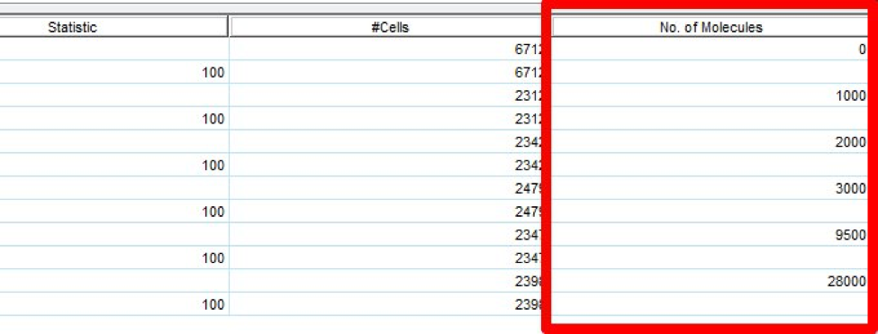 Figure 1. Sample window, showing new keyword column.
- In the workspace, add the appropriate values to the “No. of Molecules” keyword cells. (These should be known values provided by the manufacturer, for example 8,000, 16,000, 64,000, and so on.)
- Open the sample representing the calibration blank. (This establishes the background.)
- Change the plot to a histogram with the primary channel on the X-axis.
- Create a ranged gate on the modal (peak) population.
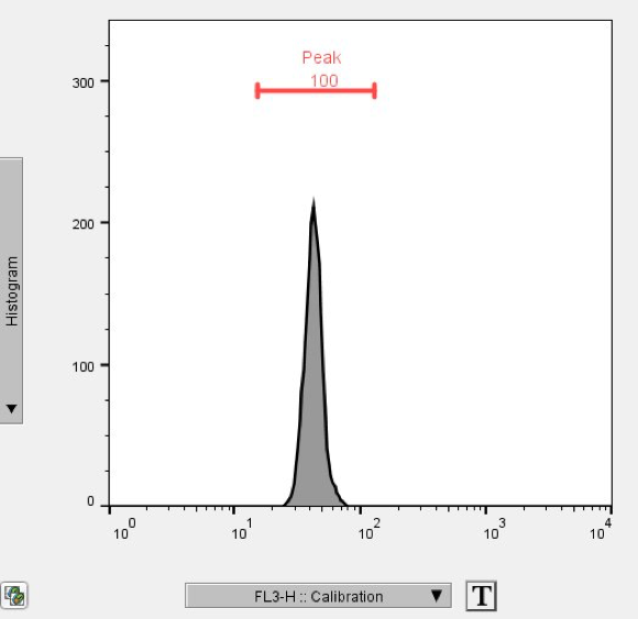 Figure 2. Graph window, showing a ranged gate on the histogram’s modal population.
- Copy the gate to the group (Command + Control + Shift + G).
- Move the ranged gates in the remaining samples to their appropriate positions.
- Add the median or geometric mean statistic (MFI) to one of the gated populations, and copy it to the group.
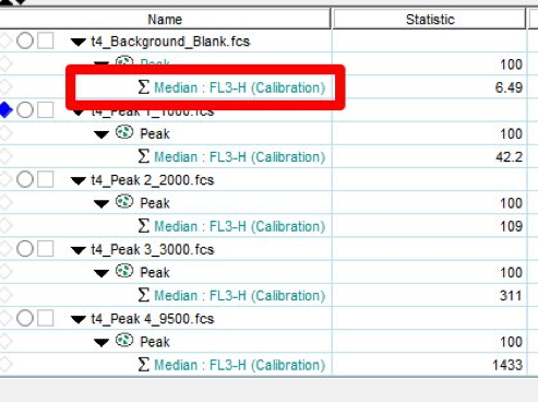 Figure 3. Sample window, showing the median.
- Open the Table Editor.
- Drag in the MFI statistic node into the Table Editor.
- Click the Edit tab. From the Columns band, select Add Column.
- In the Add Column dialog window, click the Keyword tab.
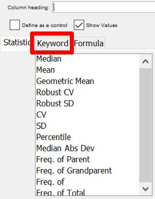 Figure 4. Add Column dialog, showing the Keyword tab.
- Select the keyword you added in Step 2 from the list of keywords in the left pane, and click OK.
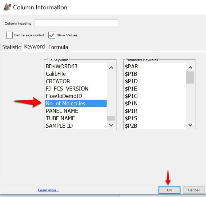 Figure 5. Add Column dialog, showing the File Keywords pane.
- The Table Editor should now have two entries, the MFI statistic and the “No. of Molecules” keyword.
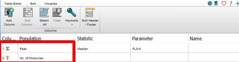 Figure 6. Table Editor, showing the original and new entry.
- In the Table Editor, highlight both entries.
- Click the Visualize tab. In the Plots band, click the Correlation Plot button.
- Ensure the target fluorochrome is on the X-axis and the “No. of Molecules” keyword is on the Y. (If they’re reversed, simply click Transpose Axes.)
- Note the slope of the line and the intercept. (You can save the image, or leave the plot open.)
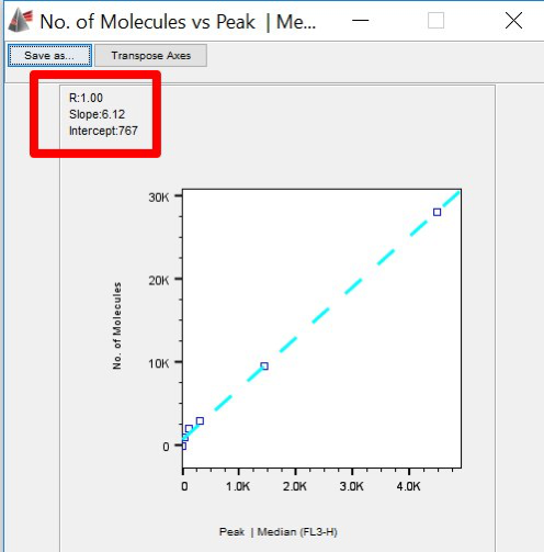 Figure 7. Correlation Plot, showing slope and intercept.
- In the workspace, right-click on a sample.
- From the drop-down menu, select Derive Parameters.
- In the Derive Parameters menu, enter a name for the parameter (for example, the No. Molecules parameter—FITC).
- Just below the plot, in the formula panel, click Insert Reference.
- Select the parameter used for the calibration (for example, FITC).
- Click the Multiply button, or add an asterisk to the nascent expression.
- Enter the slope of the line from Step 19.
-
Click the “+” button, and add the intercept from Step 19.
The derived parameter should equal the definition of a line, y = mx + b, where:
- y is the derived parameter,
- m is the slope,
- x is the parameter being used to measure the number of molecules, and
- b is the intercept.
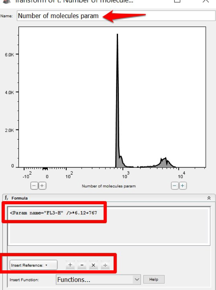 Figure 8. Derive Parameters window, showing the parameter definition.
- Click OK. (An a/b symbol appears beneath your sample.)
- Copy the derived parameter to the All Samples group. Select a sample that you want the number of molecules for.
- Right-click, and select Add Statistic from the drop-down menu.
- From the panel on the left, select Median or Geometric Mean, and choose the Derived parameter from the panel on the right.
- Click OK.
- Copy the statistic to the desired group or gates.
- The workspace’s Statistic column now displays the number of molecules on the surface of the cells for cells in that gate.
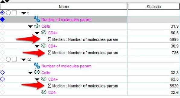 Figure 9. Samples pane, showing the new parameter.